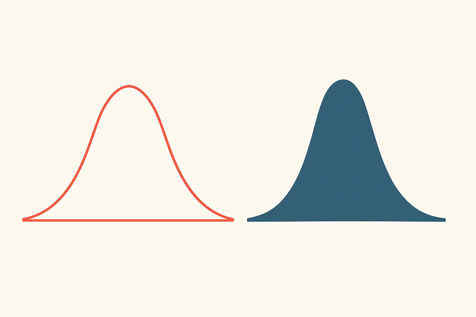
Your Shapiro-Wilk came back at p = .003, your submission is in five weeks, and it feels as though eighteen months of data collection has just been invalidated. It has not been. A failed normality test is one of the most routine events in applied research, it has four well-established routes forward, and at least one of them usually costs you nothing but a paragraph. What it does cost, if you handle it badly, is credibility — because the wrong response to a failed assumption is the one an examiner spots fastest.
Here is the whole recovery, in order: confirm what you actually tested, read the result correctly for your sample size, choose a route, and write it up so the switch reads as a decision rather than a rescue.
Step 1: Confirm you tested the right thing
Before anything else, check what you fed the test, because a meaningful share of “failed normality” results are testing the wrong quantity.
- For a group comparison, the assumption concerns the distribution of the outcome within each group, not the pooled dataset. Two perfectly normal groups with different means look decisively non-normal when combined. Split the file by group and re-run.
- For a regression, the assumption concerns the residuals, not the raw predictors or the raw outcome. Testing your predictor variables for normality is a very common and entirely unnecessary detour; regression does not assume they are normal.
- Check for data-entry damage first. A single impossible value — an age of 250, a 1-to-5 item coded 55 — will break normality on its own and will also be quietly corrupting every other statistic in your chapter.
If re-running on the correct quantity resolves it, you have lost twenty minutes and nothing else.
Step 2: Read the output correctly for your sample size
In SPSS the path is Analyze → Descriptive Statistics → Explore → Plots → Normality plots with tests, which returns both tests plus the visual diagnostics.
Which test to read depends on your N. Following Mishra and colleagues, writing in the Annals of Cardiac Anaesthesia in 2019 from the Department of Biostatistics at SGPGI Lucknow: the Shapiro-Wilk test is the more appropriate method for small sample sizes, under 50, although it can also handle larger samples, while the Kolmogorov-Smirnov test is used for n of 50 or more. For both, the null hypothesis is that the data are drawn from a normally distributed population, so p > .05 means the null is not rejected and the data can be treated as normal.
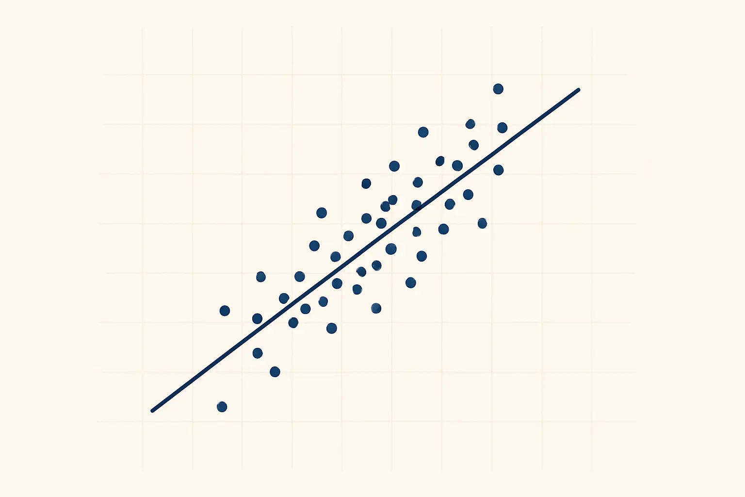
Now the part that resolves most panics. These tests are sensitive to sample size. With several hundred cases they will flag departures far too small to affect anything. That is why the same source sets out numerical criteria that scale with N, and they are worth having in front of you:
- Skewness or excess kurtosis between −1 and +1 indicates approximate normality — though this is less reliable at small to moderate sample sizes, under about 300, because it does not adjust for the standard error.
- To adjust for that, divide the skewness or excess kurtosis value by its standard error to obtain a z score. For n under 50, a z within ±1.96 is sufficient to establish normality. For 50 ≤ n < 300, the threshold is an absolute z of ±3.29.
- For n above 300, normality is judged on the histogram together with the absolute values: an absolute skewness of ≤ 2 or an absolute excess kurtosis of ≤ 4 may be used as reference values.
Note the implication for a large survey study. If you have 400 respondents and a significant Kolmogorov-Smirnov result but a skewness of 0.6 and a symmetric histogram, the defensible reading is that the significant test reflects sample size rather than a distributional problem — and you can say exactly that, with the reference values above to support it. That is Route 1, and it is the cheapest.
Step 3: Choose your route

Route 1 — Argue that the departure is trivial. Available when your N is large, the numerical indices are within the reference values, and the histogram and Q-Q plot look reasonable. Report the significant test, report the indices alongside it, note the sample-size sensitivity, and proceed with the parametric analysis. State all of this rather than omitting the failed test, which is the difference between a judgement and a concealment.
Route 2 — Switch to the non-parametric equivalent. The safest route and the one most Indian departments expect. Every common parametric test has a counterpart: Mann-Whitney U for the independent-samples t-test, Wilcoxon signed-rank for the paired t-test, Kruskal-Wallis for one-way ANOVA, Friedman for repeated-measures ANOVA, Spearman’s rho for Pearson correlation. The full mapping sits in our decision table of which statistical test to use. The cost is some statistical power and a shift in what you are testing — ranks rather than means — which your interpretation must respect.
Route 3 — Transform the variable. Where the departure has a recognisable shape, a transformation can restore normality: a logarithmic transformation for right-skewed data such as income or firm size, a square root for count data, a reciprocal for severe skew. Two conditions apply. You must apply it consistently and report it, and you must interpret your results on the transformed scale, which makes the discussion harder to write. Transform when the skew is substantive and expected in your kind of data, not as a way to make a p-value cooperate.
Route 4 — Use a robust or resampling procedure. Bootstrapped confidence intervals, available in most packages including SPSS, make far weaker distributional assumptions and let you keep the analysis you designed. Robust regression estimators serve the same purpose. This route is well accepted in the methodological literature, though it needs a sentence of explanation for a committee that has not seen it before.
Step 4: Do not do these three things
Each of them is common, each is visible, and each converts a routine assumption failure into an integrity question.
- Deleting outliers until the test passes. Legitimate outlier handling has a rule declared in advance — an impossible value, a documented measurement error, a stated criterion — and every removal is reported with its reason and the resulting N. Deleting cases until the software stops complaining is a different activity, and the shrinking N gives it away.
- Reporting the parametric result and omitting the failed check. If the check is absent from the chapter and the design obviously required one, the omission is the finding.
- Silently switching to the non-parametric test. If Chapter 3 promised a t-test and Chapter 4 delivers Mann-Whitney with no explanation, the reader assumes you went shopping for a p-value. The switch is fine; the silence is not.
Step 5: Write the paragraph
Three sentences close the issue permanently:
“Normality of the dependent variable was assessed within each group using the Shapiro-Wilk test. Scores departed significantly from normality in the intervention group (W = .92, p = .003), so the non-parametric Mann-Whitney U test was used in place of the planned independent-samples t-test. Results are reported as median and interquartile range accordingly.”
Or, for Route 1: “The Kolmogorov-Smirnov test was significant (p = .011); however, with n = 412, skewness (0.58, SE = 0.12) and excess kurtosis (−0.31, SE = 0.24) were within conventional reference values and the histogram and Q-Q plot indicated no substantive departure. The parametric analysis was therefore retained.”
Notice what both paragraphs do: they name the test, give the statistic, state the decision and state the consequence. Where each of these belongs in the chapter, and how to format the numbers, is set out in our guide to writing the results chapter. And if switching route changes what your sample can detect, the power implications are worth checking against the reasoning in our guide to calculating sample size for a thesis.
Five weeks is enough — if the writing does not become the bottleneck
The re-analysis itself is an afternoon. What actually eats the remaining weeks is the rewriting it triggers: the methodology paragraph, the results tables, the reporting conventions that change when you move from means to medians, and the discussion sentences that assumed a difference in means.
Tesify keeps your chapters structured and every citation attached to a real source as the document changes, so a switch of test in week two of five propagates as an edit rather than as a rebuild. Every analytical decision, and the responsibility for it, stays yours.
Frequently asked questions
My data is not normally distributed. Is my thesis ruined?
No. Non-normal data is routine and has four established routes forward: argue the departure is trivial, use the non-parametric equivalent, transform the variable, or use a robust or bootstrapped procedure. What matters is that you check, decide and report.
Should I use Shapiro-Wilk or Kolmogorov-Smirnov?
Shapiro-Wilk is the more appropriate method for samples under 50, though it handles larger samples too; Kolmogorov-Smirnov is used at 50 and above. Report whichever you used and be consistent across variables.
What does p greater than .05 mean in a normality test?
That the null hypothesis of normality is not rejected, so the data may be treated as normally distributed. The logic runs opposite to most tests you will run, which is why it is so often misread.
My sample is large and the test is significant. What now?
Check the numerical indices and the plots. These tests are sensitive to sample size and will flag trivial departures in large samples; if skewness and kurtosis are within the reference values, that is a reportable basis for retaining the parametric analysis.
Do I test normality on raw scores or residuals?
Residuals for regression; the outcome within each group for group comparisons. Testing raw predictor variables is unnecessary, because regression makes no normality assumption about them.
Is it acceptable to remove outliers to achieve normality?
Only under a rule declared in advance, with each removal and its reason reported. Deleting cases until the test passes is not outlier handling and is readily detected from the changing sample size.
How much power do I lose with a non-parametric test?
Some, though usually less than scholars fear, and the loss is a fair trade for a valid inference. Note it in your limitations if your sample was tight to begin with.
Which transformation should I use?
Logarithmic for right-skewed data such as income, square root for counts, reciprocal for severe skew. Apply it consistently, report it, and remember your interpretation now refers to the transformed scale.
Can I run both the parametric and non-parametric test and report both?
You can, and it is genuinely informative when both agree — it shows the conclusion is robust to the choice. Reporting both only when they disagree, and leading with the one you prefer, is not.
Does non-normality affect chi-square tests?
No. Chi-square operates on frequencies of categorical variables and carries no normality assumption. Its own requirement concerns expected cell counts.
Should I report normality testing in the results or methodology chapter?
State the planned check and the contingency in the methodology chapter, and report the actual outcome in the results chapter among the assumption checks.
Where can I read the numerical criteria myself?
Mishra and colleagues’ 2019 article on descriptive statistics and normality tests in the Annals of Cardiac Anaesthesia is open access and sets out the sample-size-dependent thresholds directly. It is short and worth reading before you write the paragraph.